
Recently I surveyed Gaussian Process Latent Variable Models (GPLVM) while getting sidetracked in one branch after another while reviewing Bayesian nonparametrics. So I thought, let’s make a blog post out of this and maybe someone else gets benefitted from my brief sprint.
GPLVM is a class of Bayesian non-parametric models. These were initially intended for dimension reduction of high dimensional data. In the last two decades, this field has grown a lot, and now it has several applications. There is a very concise recent survey paper on GPLVMs [1].
Schematic of GGLVM [1].
Key Idea: Let us assume each observed variable ( ) can be written as the sum of some latent variable (
 ) and noise (
 ). These latent variables can be thought of as functional variables
  (.), and are the noise-free form of observed variables. To infer the latent variables, GPLVM assumes that the functional variables are generated by GP from some low dimensional latent variables.
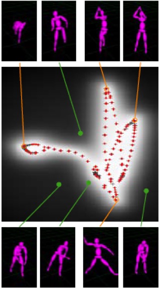
An interesting application in Motion Capture: The idea is to capture different motion sequences: a walk cycle, a jump shot, and a baseball pitch.
Figure source [2]
In the above figure, the learning process estimates a 2D position x associated with every training pose, and the plus signs (+) indicate positions of the original training points in the 2D space.
Red points indicate training poses included in the training set. Some of the original poses shown are connected to their 2D positions by orange lines. Additionally, some novel poses are shown, connected by green lines to their locations in the 2D plot [2].
Note that the new poses extrapolate from the original poses sensibly and that the original poses have been arranged so that similar poses are nearby in the 2D space. In the middle, there is a grayscale likelihood plot for each position x. Observe that points are more likely if they lie near or between similar training poses [2].
Isn’t that awesome?
Model (Involves some Math and Stat):
Consider  be the original data matrix and
  be its low dimensional representation, with
  . The schematic shown earlier can be translated in the following mathematical form,
(1) 
where  and
and  is the non-linear function with GP prior as,
  .The marginal likelihood
  can be obtained by Bayes’ theorem and integrating out ,
(2) 
Here  contains hyperparameters from the Kernel
  together with
  ,and
,and  is the
 column of .
Now we maximize the marginal likelihood with respect to and ,
(3) 
Why GPLVM over other methods?
- Firstly, the non-linear kernels in GPLVM could have considerable advantages to learn non-linear functions from the input space. It has been shown that GPLVM has a strong link with Kernel Principal Components Analysis (KPCA) [3] which is a prevalent Dimension Reduction method. The authors in [2] call this Probabilistic KPCA since it is based on a probability model and the sample covariance matrix is now replaced by the kernel.
- Secondly, there is no assumption on the projection function or the data distribution which makes it a nonparametric approach and quite flexible to deal with large and complex data sets.
References:
[1] Li, Ping, and Songcan Chen. “A review on Gaussian process latent variable models.” CAAI Transactions on Intelligence Technology 1.4 (2016): 366-376.
[2] Grochow, Keith, et al. “Style-based inverse kinematics.” ACM transactions on graphics (TOG). Vol. 23. No. 3. ACM, 2004.
[3] Schölkopf, Bernhard, Alexander Smola, and Klaus-Robert Müller. “Nonlinear component analysis as a kernel eigenvalue problem.” Neural computation 10.5 (1998): 1299-1319.